% **Blog post code introduction**
%
% Congrats on activating the "All cells" option in this interactive blog post =D
%
% Below, several new HTML blocks have appears prior to the figures, displaying the Octave/MATLAB code that was used to generate the figures in this blog post.
%
% If you want to reproduce the data on your own local computer, you simply need to have qMRLab installed in your Octave/MATLAB path and run the "startup.m" file, as is shown below.
%
% If you want to get under the hood and modify the code right now, you can do so in the Jupyter Notebook of this blog post hosted on MyBinder. The link to it is in the introduction above.
Variable Flip Angle T1 Mapping
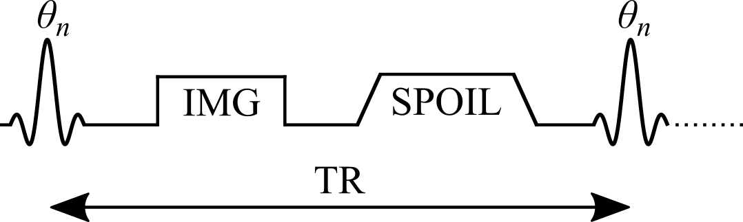
Variable flip angle (VFA) T1 mapping (Christensen et al. 1974; Gupta 1977; Fram et al. 1987), also known as Driven Equilibrium Single Pulse Observation of T1 (DESPOT1) (Homer & Beevers 1985; Deoni et al. 2003), is a rapid quantitative T1 measurement technique that is widely used to acquire 3D T1 maps (e.g. whole-brain) in a clinically feasible time. VFA estimates T1 values by acquiring multiple spoiled gradient echo acquisitions, each with different excitation flip angles (θn for n = 1, 2, .., N and θi ≠ θj). The steady-state signal of this pulse sequence (Figure 1) uses very short TRs (on the order of magnitude of 10 ms) and is very sensitive to T1 for a wide range of flip angles.
VFA is a technique that originates from the NMR field, and was adopted because of its time efficiency and the ability to acquire accurate T1 values simultaneously for a wide range of values (Christensen et al. 1974; Gupta 1977). For imaging applications, VFA also benefits from an increase in SNR because it can be acquired using a 3D acquisition instead of multislice, which also helps to reduce slice profile effects. One important drawback of VFA for T1 mapping is that the signal is very sensitive to inaccuracies in the flip angle value, thus impacting the T1 estimates. In practice, the nominal flip angle (i.e. the value set at the scanner) is different than the actual flip angle experienced by the spins (e.g. at 3.0 T, variations of up to ±30%), an issue that increases with field strength. VFA typically requires the acquisition of another quantitative map, the transmit RF amplitude (B1+, or B1 for short), to calibrate the nominal flip angle to its actual value because of B1 inhomogeneities that occur in most loaded MRI coils (Sled & Pike 1998). The need to acquire an additional B1 map reduces the time savings offered by VFA over saturation-recovery techniques, and inaccuracies/imprecisions of the B1 map are also propagated into the VFA T1 map (Boudreau et al. 2017; Lee et al. 2017).
Figure 1. Simplified pulse sequence diagram of a variable flip angle (VFA) pulse sequence with a gradient echo readout. TR: repetition time, θn: excitation flip angle for the nth measurement, IMG: image acquisition (k-space readout), SPOIL: spoiler gradient.
Signal Modelling
The steady-state longitudinal magnetization of an ideal variable flip angle experiment can be analytically solved from the Bloch equations for the spoiled gradient echo pulse sequence {θn–TR}:

where Mz is the longitudinal magnetization, M0 is the magnetization at thermal equilibrium, TR is the pulse sequence repetition time (Figure 1), and θn is the excitation flip angle. The Mz curves of different T1 values for a range of θn and TR values are shown in Figure 2.
Figure 2. Variable flip angle technique signal curves (Eq. 1) for three different T1 values, approximating the main types of tissue in the brain at 3T.
%% MATLAB/OCTAVE CODE
% Adds qMRLab to the path of the environment

cd ../qMRLab
startup
%% MATLAB/OCTAVE CODE
% Code used to generate the data required for Figure 4 of the blog post

clear all

%% Setup parameters
% All times are in milliseconds
% All flip angles are in degrees

TR_range = 5:5:200;

params.EXC_FA = 1:90;

%% Calculate signals
%
% To see all the options available, run `help vfa_t1.analytical_solution`

for ii = 1:length(TR_range)
    params.TR = TR_range(ii);

    % White matter
    params.T1 = 900; % in milliseconds

    signal_WM(ii,:) = vfa_t1.analytical_solution(params);

    % Grey matter
    params.T1 = 1500;  % in milliseconds
    signal_GM(ii,:) = vfa_t1.analytical_solution(params);

    % CSF
    params.T1 = 4000;  % in milliseconds
    signal_CSF(ii,:) = vfa_t1.analytical_solution(params);
end
From Figure 2, it is clearly seen that the flip angle at which the steady-state signal is maximized is dependent on the T1 and TR values. This flip angle is a well known quantity, called the Ernst angle (Ernst & Anderson 1966), which can be solved analytically from Equation 1 using properties of calculus:

The closed-form solution (Equation 1) makes several assumptions which in practice may not always hold true if care is not taken. Mainly, it is assumed that the longitudinal magnetization has reached a steady state after a large number of TRs, and that the transverse magnetization is perfectly spoiled at the end of each TR. Bloch simulations – a numerical approach at solving the Bloch equations for a set of spins at each time point – provide a more realistic estimate of the signal if the number of repetition times is small (i.e. a steady-state is not achieved). As can be seen from Figure 3, the number of repetitions required to reach a steady state not only depends on T1, but also on the flip angle; flip angles near the Ernst angle need more TRs to reach a steady state. Preparation pulses or an outward-in k-space acquisition pattern are typically sufficient to reach a steady state by the time that the center of k-space is acquired, which is where most of the image contrast resides.
Figure 3. Signal curves simulated using Bloch simulations (orange) for a number of repetitions ranging from 1 to 150, plotted against the ideal case (Equation 1 – blue). Simulation details: TR = 25 ms, T1 = 900 ms, 100 spins. Ideal spoiling was used for this set of Bloch simulations (transverse magnetization was set to 0 at the end of each TR).
%% MATLAB/OCTAVE CODE
% Code used to generate the data required for Figure 4 of the blog post

clear all

%% Setup parameters
% All times are in milliseconds
% All flip angles are in degrees

% White matter
params.T1 = 900; % in milliseconds
params.T2 = 10000;
params.TR = 25;
params.TE = 5;
params.EXC_FA = 1:90;
Nex_range = 1:1:150;

%% Calculate signals
%
% To see all the options available, run `help vfa_t1.analytical_solution`

for ii = 1:length(Nex_range)
    params.Nex = Nex_range(ii);

    signal_analytical(ii,:) = vfa_t1.analytical_solution(params);

    [~, complex_signal] = vfa_t1.bloch_sim(params);
    signal_blochsim(ii,:) = abs(complex(complex_signal));
end
Sufficient spoiling is likely the most challenging parameter to control for in a VFA experiment. A combination of both gradient spoiling and RF phase spoiling (Zur et al. 1991; Bernstein et al. 2004) are typically recommended (Figure 4). It has also been shown that the use of very strong gradients, introduces diffusion effects (not considered in Figure 4), further improving the spoiling efficacy in the VFA pulse sequence (Yarnykh 2010).
Figure 4. Signal curves estimated using Bloch simulations for three categories of signal spoiling: (1) ideal spoiling (blue), gradient & RF Spoiling (orange), and no spoiling (green). Simulations details: TR = 25 ms, T1 = 900 ms, Te = 100 ms, TE = 5 ms, 100 spins. For the ideal spoiling case, the transverse magnetization is set to zero at the end of each TR. For the gradient & RF spoiling case, each spin is rotated by different increments of phase (2𝜋 / # of spins) to simulate complete decoherence from gradient spoiling, and the RF phase of the excitation pulse is ɸn = ɸn-1 + nɸ0 = ½ ɸ0(n2 + n + 2) (Bernstein et al. 2004) with ɸ0 = 117° (Zur et al. 1991) after each TR.
%% MATLAB/OCTAVE CODE
% Code used to generate the data required for Figure 4 of the blog post

clear all

%% Setup parameters
% All times are in milliseconds
% All flip angles are in degrees

% White matter
params.T1 = 900; % in milliseconds
params.T2 = 100;
params.TR = 25;
params.TE = 5;
params.EXC_FA = 1:90;
Nex_range = [1:9, 10:10:100];

%% Calculate signals
%
% To see all the options available, run `help vfa_t1.analytical_solution`

for ii = 1:length(Nex_range)
    params.Nex = Nex_range(ii);

    params.crushFlag = 1;

    [~, complex_signal] = vfa_t1.bloch_sim(params);
    signal_ideal_spoil(ii,:) = abs(complex_signal);


    params.inc = 117;
    params.partialDephasing = 1;
    params.partialDephasingFlag = 1;
    params.crushFlag = 0;

    [~, complex_signal] = vfa_t1.bloch_sim(params);
    signal_optimal_crush_and_rf_spoil(ii,:) = abs(complex_signal);

    params.inc = 0;
    params.partialDephasing = 0;

    [~, complex_signal] = vfa_t1.bloch_sim(params);
    signal_no_gradient_and_rf_spoil(ii,:) = abs(complex_signal);
end
Data Fitting
At first glance, one could be tempted to fit VFA data using a non-linear least squares fitting algorithm such as Levenberg-Marquardt with Eq. 1, which typically only has two free fitting variables (T1 and M0). Although this is a valid way of estimating T1 from VFA data, it is rarely done in practice because a simple refactoring of Equation 1 allows T1 values to be estimated with a linear least square fitting algorithm, which substantially reduces the processing time. Without any approximations, Equation 1 can be rearranged into the form y = mx+b (Gupta 1977):

As the third term does not change between measurements (it is constant for each θn), it can be grouped into the constant for a simpler representation:

With this rearranged form of Equation 1, T1 can be simply estimated from the slope of a linear regression calculated from Sn/sin(θn) and Sn/tan(θn) values:

If data were acquired using only two flip angles – a very common VFA acquisition protocol – then the slope can be calculated using the elementary slope equation. Figure 5 displays both Equation 1 and 4 plotted for a noisy dataset.
Figure 5. Mean and standard deviation of the VFA signal plotted using the nonlinear form (Equation 1 – blue) and linear form (Equation 4 – red). Monte Carlo simulation details: SNR = 25, N = 1000. VFA simulation details: TR = 25 ms, T1 = 900 ms.
%% MATLAB/OCTAVE CODE
% Code used to generate the data required for Figure 4 of the blog post

clear all

%% Setup parameters
% All times are in milliseconds
% All flip angles are in degrees

params.EXC_FA = [1:4,5:5:90];

%% Calculate signals
%
% To see all the options available, run `help vfa_t1.analytical_solution`

params.TR = 0.025;
params.EXC_FA = [2:9,10:5:90];

% White matter
x.M0 = 1;
x.T1 = 0.900; % in milliseconds

Model = vfa_t1;

Opt.SNR = 25;
Opt.TR = params.TR;
Opt.T1 = x.T1;

clear Model.Prot.VFAData.Mat(:,1)
Model.Prot.VFAData.Mat = zeros(length(params.EXC_FA),2);
Model.Prot.VFAData.Mat(:,1) = params.EXC_FA';
Model.Prot.VFAData.Mat(:,2) = Opt.TR;

for jj = 1:1000
    [FitResult{jj}, noisyData{jj}] = Model.Sim_Single_Voxel_Curve(x,Opt,0);
    fittedT1(jj) = FitResult{jj}.T1;
    noisyData_array(jj,:) = noisyData{jj}.VFAData;
    noisyData_array_div_sin(jj,:) = noisyData_array(jj,:) ./ sind(Model.Prot.VFAData.Mat(:,1))';
    noisyData_array_div_tan(jj,:) = noisyData_array(jj,:) ./ tand(Model.Prot.VFAData.Mat(:,1))';
end

for kk=1:length(params.EXC_FA)
    data_mean(kk) = mean(noisyData_array(:,kk));
    data_std(kk) = std(noisyData_array(:,kk));

    data_mean_div_sin(kk) = mean(noisyData_array_div_sin(:,kk));
    data_std_div_sin(kk) = std(noisyData_array_div_sin(:,kk));

    data_mean_div_tan(kk) = mean(noisyData_array_div_tan(:,kk));
    data_std_div_tan(kk) = std(noisyData_array_div_tan(:,kk));
end


%% Setup parameters
% All times are in milliseconds
% All flip angles are in degrees

params_highres.EXC_FA = [2:1:90];

%% Calculate signals
%
% To see all the options available, run `help vfa_t1.analytical_solution`

params_highres.TR = params.TR * 1000; % in milliseconds

% White matter
params_highres.T1 = x.T1*1000; % in milliseconds

signal_WM = vfa_t1.analytical_solution(params_highres);
signal_WM_div_sin = signal_WM ./ sind(params_highres.EXC_FA);
signal_WM_div_tan = signal_WM ./ tand(params_highres.EXC_FA);
There are two important imaging protocol design considerations that should be taken into account when planning to use VFA: (1) how many and which flip angles to use to acquire VFA data, and (2) correcting inaccurate flip angles due to transmit RF field inhomogeneity. Most VFA experiments use the minimum number of required flip angles (two) to minimize acquisition time. For this case, it has been shown that the flip angle choice resulting in the best precision for VFA T1 estimates for a sample with a single T1 value (i.e. single tissue) are the two flip angles that result in 71% of the maximum possible steady-state signal (i.e. at the Ernst angle) (Deoni et al. 2003; Schabel & Morrell 2009).
Time allowing, additional flip angles are often acquired at higher values and in between the two above, because greater signal differences between tissue T1 values are present there (e.g. Figure 2). Also, for more than two flip angles, Equations 1 and 4 do not have the same noise weighting for each fitting point, which may bias linear least-square T1 estimates at lower SNRs. Thus, it has been recommended that low SNR data should be fitted with either Equation 1 using non-linear least-squares (slower fitting) or with a weighted linear least-squares form of Equation 4 (Chang et al. 2008).
Accurate knowledge of the flip angle values is very important to produce accurate T1 maps. Because of how the RF field interacts with matter (Sled & Pike 1998), the excitation RF field (B1+, or B1 for short) of a loaded RF coil results in spatial variations in intensity/amplitude, unless RF shimming is available to counteract this effect (not common at clinical field strengths). For quantitative measurements like VFA which are sensitive to this parameter, the flip angle can be corrected (voxelwise) relative to the nominal value by multiplying it with a scaling factor (B1) from a B1 map that is acquired during the same session:

B1 in this context is normalized, meaning that it is unitless and has a value of 1 in voxels where the RF field has the expected amplitude (i.e. where the nominal flip angle is the actual flip angle). Figure 6 displays fitted VFA T1 values from a Monte Carlo dataset simulated using biased flip angle values, and fitted without/with B1 correction.
Figure 6. Mean and standard deviations of fitted VFA T1 values for a set of Monte Carlo simulations (SNR = 100, N = 1000), simulated using a wide range of biased flip angles and fitted without (blue) or with (red) B1 correction. Simulation parameters: TR = 25 ms, T1 = 900 ms, θnominal = 6° and 32° (optimized values for this TR/T1 combination). Notice how even after B1 correction, fitted T1 values at B1 values far from the nominal case (B1 = 1) exhibit larger variance, as the actual flip angles of the simulated signal deviate from the optimal values for this TR/T1 (Deoni et al. 2003).
%% MATLAB/OCTAVE CODE
% Code used to generate the data required for Figure 4 of the blog post

clear all

%% Setup parameters
% All times are in seconds
% All flip angles are in degrees

params.TR = 0.025; % in seconds

% White matter
params.T1 = 0.900; % in seconds

% Calculate optimal flip angles for a two flip angle VFA experiment (for this T1 and TR)
% The will be the nominal flip angles (the flip angles assumed by the "user", before a
% "realistic"B1 bias is applied)

nominal_EXC_FA = vfa_t1.find_two_optimal_flip_angles(params); % in degrees
disp('Nominal flip angles:')
disp(nominal_EXC_FA)

% Range of B1 values biasing the excitation flip angle away from their nominal values
B1Range = 0.1:0.1:2;

x.M0 = 1;
x.T1 = params.T1; % in seconds

Model = vfa_t1;

Model.voxelwise = 1;

Opt.SNR = 100;
Opt.TR = params.TR;
Opt.T1 = x.T1;

% Monte Carlo signal simulations
for ii = 1:1000
    for jj = 1:length(B1Range)
        B1 = B1Range(jj);
        actual_EXC_FA = B1 * nominal_EXC_FA;

        params.EXC_FA = actual_EXC_FA;

        clear Model.Prot.VFAData.Mat(:,1)
        Model.Prot.VFAData.Mat = zeros(length(params.EXC_FA),2);
        Model.Prot.VFAData.Mat(:,1) = params.EXC_FA';
        Model.Prot.VFAData.Mat(:,2) = Opt.TR;

        [FitResult{ii,jj}, noisyData{ii,jj}] = Model.Sim_Single_Voxel_Curve(x,Opt,0);
        noisyData_array(ii,jj,:) = noisyData{ii,jj}.VFAData;
    end
end
%
Model = vfa_t1;

Model.voxelwise = 1;

FlipAngle = nominal_EXC_FA';
TR = params.TR .* ones(size(FlipAngle));

Model.Prot.VFAData.Mat = [FlipAngle TR];

data.VFAData(:,:,1,1) = noisyData_array(:,:,1);
data.VFAData(:,:,1,2) = noisyData_array(:,:,2);
data.Mask = repmat(ones(size(B1Range)),[size(noisyData_array,1),1]);

data.B1map = repmat(ones(size(B1Range)),[size(noisyData_array,1),1]);
FitResults_noB1Correction = FitData(data,Model,0);

data.B1map = repmat(B1Range,[size(noisyData_array,1),1]);
FitResults_withB1Correction = FitData(data,Model,0);

%%
%

mean_T1_noB1Correction = mean(FitResults_noB1Correction.T1);
mean_T1_withB1Correction = mean(FitResults_withB1Correction.T1);
std_T1_noB1Correction = std(FitResults_noB1Correction.T1);
std_T1_withB1Correction = std(FitResults_withB1Correction.T1);
Figure 7 displays an example VFA dataset and a B1 map in a healthy brain, along with the T1 map estimated using a linear fit (Equations 4 and 5).
Figure 7. Example variable flip angle dataset and B1 map of a healthy adult brain (left). The relevant VFA protocol parameters used were: TR = 15 ms, θnominal = 3° and 20°. The T1 map (right) was fitted using a linear regression (Equations 4 and 5).
%% MATLAB/OCTAVE CODE
% Download variable flip angle brain MRI data for Figure 7 of the blog post

cmd = ['curl -L -o vfa_brain.zip https://osf.io/wj6eg/download/'];
[STATUS,MESSAGE] = unix(cmd);
unzip('vfa_brain.zip');
%% MATLAB/OCTAVE CODE
% Code used to generate the data required for Figure 5 of the blog post

clear all

% Load data into environment, and rotate mask to be aligned with IR data
load('VFAData.mat');
load('B1map.mat');
load('Mask.mat');

% Format qMRLab vfa_t1 model parameters, and load them into the Model object
Model = vfa_t1;
FlipAngle = [    3;     20];
TR        = [0.015; 0.0150];


Model.Prot.VFAData.Mat = [FlipAngle, TR];

% Format data structure so that they may be fit by the model
data = struct();
data.VFAData= double(VFAData);
data.B1map= double(B1map);
data.Mask= double(Mask);

FitResults = FitData(data,Model,0); % The '0' flag is so that no wait bar is shown.
%% MATLAB/OCTAVE CODE
% Code used to re-orient the images to make pretty figures, and to assign variables with the axis lengths.

T1_map = imrotate(FitResults.T1.*Mask,-90);
T1_map(T1_map>5)=0;
T1_map = T1_map*1000; % Convert to ms

xAxis = [0:size(T1_map,2)-1];
yAxis = [0:size(T1_map,1)-1];

% Raw MRI data at different TI values
FA_03 = imrotate(squeeze(VFAData(:,:,:,1).*Mask),-90);
FA_20 = imrotate(squeeze(VFAData(:,:,:,2).*Mask),-90);
B1map = imrotate(squeeze(B1map.*Mask),-90);
Benefits and Pitfalls
It has been well reported in recent years that the accuracy of VFA T1 estimates is very sensitive to pulse sequence implementations (Stikov et al. 2015; Lutti & Weiskopf 2013; Baudrexel et al. 2018), and as such is less robust than the gold standard inversion recovery technique. In particular, the signal bias resulting from insufficient spoiling can result in inaccurate T1 estimates of up to 30% relative to inversion recovery estimated values (Stikov et al. 2015). VFA T1 map accuracy and precision is also strongly dependent on the quality of the measured B1 map (Lee et al. 2017), which can vary substantially between implementations (Boudreau et al. 2017). Modern rapid B1 mapping pulse sequences are not as widely available as VFA, resulting in some groups attempting alternative ways of removing the bias from the T1 maps like generating an artificial B1 map through the use of image processing techniques (Liberman et al. 2014) or omitting B1 correction altogether (Yuan et al. 2012). The latter is not recommended, because most MRI scanners have default pulse sequences that, with careful protocol settings, can provide B1 maps of sufficient quality very rapidly (Boudreau et al. 2017; Wang et al. 2005; Samson et al. 2006).
Despite some drawbacks, VFA is still one of the most widely used T1 mapping methods in research. Its rapid acquisition time, rapid image processing time, and widespread availability makes it a great candidate for use in other quantitative imaging acquisition protocols like quantitative magnetization transfer imaging (Yarnykh 2002; Cercignani et al. 2005) and dynamic contrast enhanced imaging (Sung et al. 2013; Li et al. 2018).
Works Cited
Baudrexel, S. et al., 2018. T1 mapping with the variable flip angle technique: A simple correction for insufficient spoiling of transverse magnetization. Magn. Reson. Med., 79(6), pp.3082–3092.
Bernstein, M., King, K. & Zhou, X., 2004. Handbook of MRI Pulse Sequences, Elsevier.
Boudreau, M. et al., 2017. B1 mapping for bias-correction in quantitative T1 imaging of the brain at 3T using standard pulse sequences. J. Magn. Reson. Imaging, 46(6), pp.1673–1682.
Cercignani, M. et al., 2005. Three-dimensional quantitative magnetisation transfer imaging of the human brain. Neuroimage, 27(2), pp.436–441.
Chang, L.-C. et al., 2008. Linear least-squares method for unbiased estimation of T1 from SPGR signals. Magn. Reson. Med., 60(2), pp.496–501.
Christensen, K.A. et al., 1974. Optimal determination of relaxation times of fourier transform nuclear magnetic resonance. Determination of spin-lattice relaxation times in chemically polarized species. J. Phys. Chem., 78(19), pp.1971–1977.
Deoni, S.C.L., Rutt, B.K. & Peters, T.M., 2003. Rapid combined T1 and T2 mapping using gradient recalled acquisition in the steady state. Magn. Reson. Med., 49(3), pp.515–526.
Ernst, R.R. & Anderson, W.A., 1966. Application of Fourier Transform Spectroscopy to Magnetic Resonance. Rev. Sci. Instrum., 37(1), pp.93–102.
Fram, E.K. et al., 1987. Rapid calculation of T1 using variable flip angle gradient refocused imaging. Magn. Reson. Imaging, 5(3), pp.201–208.
Gupta, R.K., 1977. A new look at the method of variable nutation angle for the measurement of spin-lattice relaxation times using fourier transform NMR. J. Magn. Reson., 25(1), pp.231–235.
Homer, J. & Beevers, M.S., 1985. Driven-equilibrium single-pulse observation of T1 relaxation. A reevaluation of a rapid “new” method for determining NMR spin-lattice relaxation times. J. Magn. Reson., 63(2), pp.287–297.
Lee, Y., Callaghan, M.F. & Nagy, Z., 2017. Analysis of the Precision of Variable Flip Angle T1 Mapping with Emphasis on the Noise Propagated from RF Transmit Field Maps. Front. Neurosci., 11, p.106.
Liberman, G., Louzoun, Y. & Ben Bashat, D., 2014. T1 mapping using variable flip angle SPGR data with flip angle correction. J. Magn. Reson. Imaging, 40(1), pp.171–180.
Li, Z.F. et al., 2018. A simple B1 correction method for dynamic contrast-enhanced MRI. Phys. Med. Biol., 63(16), p.16NT01.
Lutti, A. & Weiskopf, N., 2013. Optimizing the accuracy of T1 mapping accounting for RF non-linearities and spoiling characteristics in FLASH imaging. In Proceedings of the 21st Annual Meeting of ISMRM, Salt Lake City, Utah, USA. p. 2478.
Samson, R.S. et al., 2006. A simple correction for B1 field errors in magnetization transfer ratio measurements. Magn. Reson. Imaging, 24(3), pp.255–263.
Schabel, M.C. & Morrell, G.R., 2009. Uncertainty in T1 mapping using the variable flip angle method with two flip angles. Phys. Med. Biol., 54(1), pp.N1–8.
Sled, J.G. & Pike, G.B., 1998. Standing-wave and RF penetration artifacts caused by elliptic geometry: an electrodynamic analysis of MRI. IEEE Trans. Med. Imaging, 17(4), pp.653–662.
Stikov, N. et al., 2015. On the accuracy of T1 mapping: Searching for common ground. Magn. Reson. Med., 73(2), pp.514–522.
Sung, K., Daniel, B.L. & Hargreaves, B.A., 2013. Transmit B1+ field inhomogeneity and T1 estimation errors in breast DCE-MRI at 3 tesla. J. Magn. Reson. Imaging, 38(2), pp.454–459.
Wang, J., Qiu, M. & Constable, R.T., 2005. In vivo method for correcting transmit/receive nonuniformities with phased array coils. Magn. Reson. Med., 53(3), pp.666–674.
Yarnykh, V.L., 2010. Optimal radiofrequency and gradient spoiling for improved accuracy of T1 and B1 measurements using fast steady-state techniques. Magn. Reson. Med., 63(6), pp.1610–1626.
Yarnykh, V.L., 2002. Pulsed Z-spectroscopic imaging of cross-relaxation parameters in tissues for human MRI: theory and clinical applications. Magn. Reson. Med., 47(5), pp.929–939.
Yuan, J. et al., 2012. Quantitative evaluation of dual-flip-angle T1 mapping on DCE-MRI kinetic parameter estimation in head and neck. Quant. Imaging Med. Surg., 2(4), pp.245–253.
Zur, Y., Wood, M.L. & Neuringer, L.J., 1991. Spoiling of transverse magnetization in steady-state sequences. Magn. Reson. Med., 21(2), pp.251–263.
# PYTHON CODE

display(HTML(
    '<style type="text/css">'
    '.output_subarea {'
        'display: block;'
        'margin-left: auto;'
        'margin-right: auto;'
    '}'
    '.blog_body {'
        'line-height: 2;'
        'font-family: timesnewroman;'
        'font-size: 18px;'
        'margin-left: 0px;'
        'margin-right: 0px;'
    '}'
    '.biblio_body {'
        'line-height: 1.5;'
        'font-family: timesnewroman;'
        'font-size: 18px;'
        'margin-left: 0px;'
        'margin-right: 0px;'
    '}'
    '.note_body {'
        'line-height: 1.25;'
        'font-family: timesnewroman;'
        'font-size: 18px;'
        'margin-left: 0px;'
        'margin-right: 0px;'
        'color: #696969'
    '}'
    '.figure_caption {'
        'line-height: 1.5;'
        'font-family: timesnewroman;'
        'font-size: 16px;'
        'margin-left: 0px;'
        'margin-right: 0px'
    '</style>'
))