T_1𝞺 Mapping

T₁ relaxation time at clinical fields (1.5 or 3 T) probes the molecular motional processes in the MHz range (e.g. 64 or 128 MHz). To measure such processes in the kHz range, while still performing the experiment at clinical fields, we can use T_1𝞺 relaxation (Redfield 1955). In a T_1𝞺 relaxation experiment, a spin-lock pulse, ω₁, is applied in the rotating frame, proportional to the B₁ field (ω₁ = ɣB₁). The result is that the spins rotate around the spin-lock pulse in the rotating frame, similar to T₁ relaxation, where the spins rotate around B₀. Due to that similarity to the T₁ relaxation experiment, T_1𝞺 is known as the spin-lattice relaxation time in the rotating frame (Jones 1966). T_1𝞺 has previously been used with ω₁ = 1 to 20 kHz to acquire information about T₁ relaxation times at lower field strengths using a clinical system operating at 0.15 T (Santyr et al. 1989), which had more available signal than imaging at 0.001 T as had previously been done (Koenig & Brown 1984).

The T_1𝞺 experiment is also similar to the T₂ experiment; the typical implementation is to precede a T₂ experiment with a T_1𝞺 preparation. The applied spin-lock pulse suspends any relaxation mechanisms that occur at or below the specific spin-lock pulse frequency, and once the spin-lock pulse is removed, these relaxation mechanisms will proceed (Borthakur et al. 2006). T₂ relaxation is sensitive to water molecule diffusion, dipole-dipole interaction and local field inhomogeneities. T_1𝞺 relaxation is sensitive to the same processes as T₂ relaxation, along with chemical exchange processes and slow rotational motions of protons associated with large macromolecules (Akella et al. 2001; Mlynárik et al. 2004; Duvvuri et al. 1997). The spin-lock pulses can be used, for example, to suppress the effect of dipolar interaction, and as a result, the T_1𝞺 relaxation times are longer than T₂ relaxation times (Regatte & Schweitzer 2008). In this example, the difference between the T_1𝞺 and T₂ relaxation times is driven by the amount of water-macromolecule interaction (Duvvuri et al. 1997).

T_1𝞺 has been applied to many clinical applications including the breast (Santyr et al. 1989; Fairbanks et al. 1995), heart (Dixon et al. 1996; Muthupillai et al. 2004; Witschey et al. 2012; Kamesh Iyer et al. 2019), liver (Allkemper et al. 2014), brain (Aronen et al. 1999; Borthakur et al. 2008; Haris et al. 2011; Michaeli et al. 2006), and musculoskeletal systems (Li et al. 2007; Keenan et al. 2015; Johannessen et al. 2006). A particularly interesting application of T_1𝞺 is T_1𝞺 dispersion, where the spin-lock frequency is systematically varied to affect different mechanisms of relaxation in tissue. The information acquired is comparable to T₁ dispersion studies; however, because only B₁ is varied, the data can be acquired using any MRI system. The major challenge preventing adoption of T_1𝞺 methods is that the spin-lock pulse frequencies are limited by the specific absorption rate (SAR) (Wheaton et al. 2004).

Figure 1. Simplified diagram of a T_1𝞺 Spin-Lock pulse sequence illustrating the tip-down RF pulse, spin-lock pulse (θ_y), the tip-up RF pulse and the crusher to dephase residual signal in the transverse plane.

Signal Modelling

In the T_1𝞺 experiment (Figure 1), a spin-lock pulse is applied at a frequency, ω₁, which will affect some relaxation processes. The spins precess around the spin-lock axis in the rotating frame (Figure 2a), and when the spin-lock pulse is removed, the spins return to their original orientation. The spin-lock pulse will sensitize measurements to processes at or around the time scale 1/ω₁. The spin-lock frequency is typically varied from 100-500 Hz at clinical field strengths. T_1𝞺 relaxation can be characterized by:

where TSL is the time of the spin-lock pulse and S₀ is a constant, which is independent of TSL. The TSL varies from approximately 2 ms to 100 ms, depending on the tissue of interest, and it is recommended that a minimum of four TSL values be used.

A simple T_1𝞺 preparation applies 90-degree RF pulse to tip into the M_xy plane, followed by the spin-lock pulse applied parallel to the magnetization for duration TSL, then another 90-degree RF pulse is applied to flip the magnetization back to the longitudinal direction, and a crusher is used to dephase residual signal in the transverse plane Figure 1. However, there are several potential artifacts resulting from this simple sequence. A complete signal model of this sequence results in the following:

where α is the actual tip-up/tip-down RF pulse flip angle, θ is the total flip angle during spin locking (proportional to TSL), and T_2𝞺 is the magnetization decay rate in the plane perpendicular to the spin-locking RF pulse. T_2𝞺 is not regularly studied and is beyond the scope of this discussion.

Figure 2. Rotating frame representation of the T_1𝞺 experiment (a). In the rotating frame of reference, the spins experience an effective RF field, ω_eff. Typically, the spin-lock pulse is applied on-resonance and the spins experience ω_eff = ω₁ = ɣB₁. If an off-resonance pulse is used, the spins experience ω_eff = Δ + ω₁, where Δ is the off-resonance component. The timing diagram (b) of a simplified T_1𝞺 experiment illustrating the suspension of some relaxation processes during the application of the spin-lock pulse, θ_y. After the spin-lock pulse is removed, the magnetization relaxes as a free induction decay, FID.

For example, it is well documented that with this pulse sequence, B₀ and B₁ inhomogeneities can cause oscillations in the relaxation decay curve (Chen et al. 2011; Witschey et al. 2007). Simply reversing the amplitude or phase of the second half of the spin-locking pulse to create a rotary echo (Solomon 1959) is insufficient to address the B₁ inhomogeneities (Chen 2015; Charagundla et al. 2003). A solution is to use phase cycling to address B₁ inhomogeneities, and one method acquires two data sets with opposite phase of the tip-up RF pulse, which are then subtracted from each other (Chen et al. 2011). The resulting longitudinal magnetization is:

And as result, the monoexponential decay model (Eq. 1) can be used. It should be noted that because the method requires two data sets, the scan time is doubled. However, there is no scan time penalty to incorporate this method in the 3D sequence designed by Li et al. (Li et al. 2008). Finally, to address the effect of B₀ and B₁ inhomogeneities simultaneously, it is possible to combine a composite RF pulse (Dixon et al. 1996) with the phase cycling method (Chen et al. 2011) or use the method proposed by Witschey et al. (Witschey et al. 2007) that uses four different pulse clusters: a conventional spin-lock, a B₁ insensitive spin-lock (Chen 2015; Charagundla et al. 2003), a ΔB₀ insensitive spin-lock (Zeng et al. 2006), and finally a ΔB₀ and B₁ insensitive spin-lock, which aligns the final magnetization along the z-axis.

Data Fitting

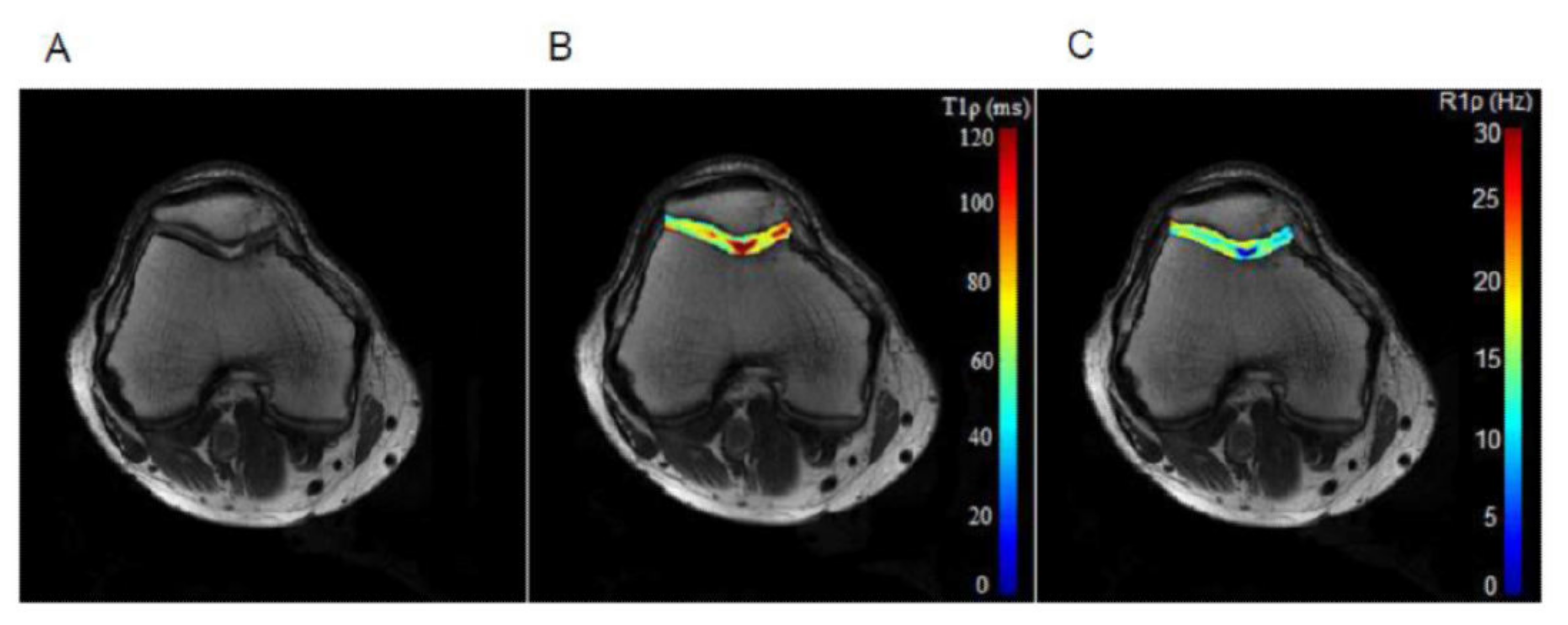
T_1𝞺 relaxation is typically modeled and fitted using a monoexponential, Eq. 1, similar to T₂ relaxation, and a linear least squares fitting algorithm can be used. However, depending on the sequence, the signal model may need additional complexity to account for the effect of T_2𝞺 relaxation, as in Eq. 2 (Charagundla et al. 2003). An example T_1𝞺 relaxation map of cartilage in the knee is shown in Figure 3. The model used could also account for chemical exchange (Chopra et al. 1984) and Cobb et al (Cobb et al. 2014).

Figure 3. An example T_1𝞺 relaxation map of cartilage in the knee, using a spin-lock frequency of 350 Hz, five TSLs linearly spaced from 2-82 ms, and TR/TE 3300 ms/10 ms. Reproduced with permission from (Wang et al. 2015).

The linear least squares fit is appropriate when the SNR is sufficiently high. In the case of low SNR, large bias appears with both the linear and non-linear fit to Eq. 1. Several approaches have been developed to fit low SNR T₂, which can also be applied to low SNR T_1𝞺 (Bonny et al. 1996; Raya et al. 2010; Hardy & Andersen 2009).

In the T_1𝞺 dispersion experiment, the T1ρ experiment is repeated with different spin-lock pulse frequencies, and T_1𝞺 relaxation is plotted against the spin-lock frequency to generate the T_1𝞺 dispersion curve. In tissues, T_1𝞺 relaxation times increase with increasing spin-lock frequencies (Duvvuri et al. 2001). The dispersion curve shape will depend on the tissue components (Duvvuri et al. 2001; Koskinen et al. 2006), and the fit to the curve can be used to characterize the tissue. For example, Koskinen et al. used a small range of spin-lock frequencies and fit the slope of 1/T_1𝞺 over the spin-lock frequency to characterize various rat organs (Koskinen et al. 1999; Koskinen et al. 2006), whereas 1/T_1𝞺 in cartilage, examined over a large range of spin-lock frequencies, was fitted using a bi-Lorentzian model (Duvvuri et al. 2001).

Benefits and Pitfalls

T_1𝞺 is able to probe small changes in the macromolecular content using clinically available equipment. By manipulating ω₁ in the spin-lock pulse, it is possible to measure, for example, exchange-dependent pH changes (Cobb et al. 2012). T_1𝞺 has been used extensively to study the musculoskeletal system, including cartilage, meniscus and interverterbral discs. T_1𝞺 relaxation may be able to distinguish tumor, healthy, and adipose tissues in the breast (Santyr et al. 1989); improve delineation of myocardial borders (Dixon et al. 1996) and detect acute myocardial injuries (Muthupillai et al. 2004); and aid in detection and assessment of liver cirrhosis (Allkemper et al. 2014). Spin-lock sequences have specifically been developed for accelerated 3D acquisition in the heart (Kamesh Iyer et al. 2019). In the brain, T_1𝞺 relaxation was used at low field (0.1 T) with contrast to identify gliomas (Aronen et al. 1999) and at higher fields (4 T) to study macromolecules (Michaeli et al. 2006). These macromolecular changes detected by T_1𝞺 in the brain (in this case at 1.5 T), may be indicative of neurodegenerative diseases such as Alzheimer’s and Parkinson’s disease (Borthakur et al. 2008; Haris et al. 2011).

The major challenge preventing T_1𝞺 from adoption is that the power deposition required by spin-locking pulses approaches the clinical SAR limits. T_1𝞺 dispersion, in particular, has limited clinical application because of power limitations from SAR concerns. There have been pulse sequence developments to overcome these challenges through the use of parallel transmit (Chen et al. 2016), partial k-space application of the spin-lock pulse (Wheaton et al. 2004), or the use of off-resonance pulses (Santyr et al. 1994), though T_1𝞺-off resonance is beyond the scope of this discussion. However, there are benefits of even very low frequency (0-400 Hz) spin-lock pulses, which are within clinical limits, to detect residual dipolar interactions in structured tissues such as oriented collagen fibers or myelinated axons (Witschey et al. 2007).

Works Cited

Akella, S.V.S. et al., 2001. Proteoglycan-induced changes in T_1𝞺-relaxation of articular cartilage at 4T. Magn. Reson. Med., 46(3), pp.419–423.

Allkemper, T. et al., 2014. Evaluation of fibrotic liver disease with whole-liver T_1𝞺 MR imaging: a feasibility study at 1.5 T. Radiology, 271(2), pp.408–415.

Aronen, H.J. et al., 1999. 3D spin-lock imaging of human gliomas. Magn. Reson. Imaging, 17(7), pp.1001–1010.

Bonny, J.M. et al., 1996. T₂ maximum likelihood estimation from multiple spin-echo magnitude images. Magn. Reson. Med., 36(2), pp.287–293.

Borthakur, A. et al., 2006. Sodium and T1rho MRI for molecular and diagnostic imaging of articular cartilage. NMR Biomed., 19(7), pp.781–821.

Borthakur, A. et al., 2008. T1rho MRI of Alzheimer’s disease. Neuroimage, 41(4), pp.1199–1205.

Charagundla, S.R. et al., 2003. Artifacts in T(1rho)-weighted imaging: correction with a self-compensating spin-locking pulse. J. Magn. Reson., 162(1), pp.113–121.

Chen, W., 2015. Errors in quantitative T1rho imaging and the correction methods. Quant. Imaging Med. Surg., 5(4), pp.583–591.

Chen, W., Takahashi, A. & Han, E., 2011. Quantitative T_1𝞺 imaging using phase cycling for B₀ and B₁ field inhomogeneity compensation. Magn. Reson. Imaging, 29(5), pp.608–619.

Chen, W., Chan, Q. & Wáng, Y.-X.J., 2016. Breath-hold black blood quantitative T1rho imaging of liver using single shot fast spin echo acquisition. Quant. Imaging Med. Surg., 6(2), pp.168–177.

Chopra, S., McClung, R.E.D. & Jordan, R.B., 1984. Rotating-frame relaxation rates of solvent molecules in solutions of paramagnetic ions undergoing solvent exchange. J. Magn. Reson., 59(3), pp.361–372.

Cobb, J.G. et al., 2012. Exchange-mediated contrast agents for spin-lock imaging. Magn. Reson. Med., 67(5), pp.1427–1433.

Cobb, J.G. et al., 2014. Exchange-mediated contrast in CEST and spin-lock imaging. Magn. Reson. Imaging, 32(1), pp.28–40.

Dixon, W.T. et al., 1996. Myocardial suppressionin vivo by spin locking with composite pulses. Magn. Reson. Med., 36(1), pp.90–94.

Duvvuri, U. et al., 1997. T_1𝞺-relaxation in articular cartilage: Effects of enzymatic degradation. Magn. Reson. Med., 38(6), pp.863–867.

Duvvuri, U. et al., 2001. Water magnetic relaxation dispersion in biological systems: the contribution of proton exchange and implications for the noninvasive detection of cartilage degradation. Proc. Natl. Acad. Sci. U.S.A., 98(22), pp.12479–12484.

Fairbanks, E.J., Santyr, G.E. & Sorenson, J.A., 1995. One-shot measurement of spin-lattice relaxation times in the off-resonance rotating frame using MR imaging, with application to breast. J. Magn. Reson. B, 106(3), pp.279–283.

Hardy, P.A. & Andersen, A.H., 2009. Calculating T₂ in images from a phased array receiver. Magn. Reson. Med., 61(4), pp.962–969.

Haris, M. et al., 2011. T1rho (T_1𝞺) MR imaging in Alzheimer’s disease and Parkinson's disease with and without dementia. J. Neurol., 258(3), pp.380–385.

Johannessen, W. et al., 2006. Assessment of human disc degeneration and proteoglycan content using T1rho-weighted magnetic resonance imaging. Spine, 31(11), pp.1253–1257.

Jones, G.P., 1966. Spin-Lattice Relaxation in the Rotating Frame: Weak-Collision Case. Phys. Rev., 148(1), pp.332–335.

Kamesh Iyer, S. et al., 2019. Accelerated free-breathing 3D T_1𝞺 cardiovascular magnetic resonance using multicoil compressed sensing. J. Cardiovasc. Magn. Reson., 21(1), p.5.

Keenan, K.E. et al., 2015. T_1𝞺 Dispersion in Articular Cartilage: Relationship to Material Properties and Macromolecular Content. Cartilage, 6(2), pp.113–122.

Koenig, S.H. & Brown, R.D., 3rd, 1984. Determinants of proton relaxation rates in tissue. Magn. Res. in Med., 1(4), pp.437–449.

Koskinen, S.K. et al., 2006. T1rho Dispersion profile of rat tissues in vitro at very low locking fields. Magn. Reson. Imaging, 24(3), pp.295–299.

Koskinen, S.K. et al., 1999. T_1𝞺 dispersion of rat tissues in vitro. Magn. Reson. Imaging, 17(7), pp.1043–1047.

Li, X. et al., 2007. In vivo T(1rho) and T(2) mapping of articular cartilage in osteoarthritis of the knee using 3 T MRI. Osteoarthritis Cartilage, 15(7), pp.789–797.

Li, X. et al., 2008. In vivo T(1rho) mapping in cartilage using 3D magnetization-prepared angle-modulated partitioned k-space spoiled gradient echo snapshots (3D MAPSS). Magn. Reson. Med., 59(2), pp.298–307.

Michaeli, S. et al., 2006. T1rho MRI contrast in the human brain: modulation of the longitudinal rotating frame relaxation shutter-speed during an adiabatic RF pulse. J. Magn. Reson., 181(1), pp.135–147.

Mlynárik, V. et al., 2004. Transverse relaxation mechanisms in articular cartilage. J. Magn. Reson., 169(2), pp.300–307.

Muthupillai, R. et al., 2004. Acute myocardial infarction: tissue characterization with T1rho-weighted MR imaging--initial experience. Radiology, 232(2), pp.606–610.

Raya, J.G. et al., 2010. T₂ measurement in articular cartilage: impact of the fitting method on accuracy and precision at low SNR. Magn. Reson. Med., 63(1), pp.181–193.

Redfield, A.G., 1955. Nuclear Magnetic Resonance Saturation and Rotary Saturation in Solids. Phys. Rev., 98(6), pp.1787–1809.

Regatte, R.R. & Schweitzer, M.E., 2008. Novel contrast mechanisms at 3 Tesla and 7 Tesla. Semin. Musculoskelet. Radiol., 12(3), pp.266–280.

Santyr, G.E., Henkelman, R.M. & Bronskill, M.J., 1989. Spin locking for magnetic resonance imaging with application to human breast. Magn. Reson. Med., 12(1), pp.25–37.

Santyr, G.E. et al., 1994. Off-resonance spin locking for MR imaging. Magn. Reson. Med., 32(1), pp.43–51

Solomon, I., 1959. Rotary Spin Echoes. Phys. Rev. Lett., 2(7), pp.301–302.

Wang, P., Block, J. & Gore, J.C., 2015. Chemical exchange in knee cartilage assessed by R_1𝞺 (1/T_1𝞺) dispersion at 3T. Magn. Reson. Imaging, 33(1), pp.38–42.

Wheaton, A.J. et al., 2004. Method for reduced SAR T1rho-weighted MRI. Magn. Reson. Med., 51(6), pp.1096–1102.

Witschey, W.R.T., 2nd et al., 2007. Artifacts in T1 rho-weighted imaging: compensation for B(1) and B(0) field imperfections. J. Magn. Reson., 186(1), pp.75–85.

Witschey, W.R.T. et al., 2012. In vivo chronic myocardial infarction characterization by spin locked cardiovascular magnetic resonance. J. Cardiovasc. Magn. Reson., 14, p.37.

Zeng, H. et al., 2006. A composite spin-lock pulse for deltaB0 + B1 insensitive T1rho measurement. In Proceedings of the 14th Annual Meeting of ISMRM, Seattle, Washington, USA. p. 2356.

# PYTHON CODE
from IPython.core.display import display, HTML
display(HTML(
    '<style type="text/css">'
    '.output_subarea {'
        'display: block;'
        'margin-left: auto;'
        'margin-right: auto;'
    '}'
    '.blog_body {'
        'line-height: 2;'
        'font-family: timesnewroman;'
        'font-size: 18px;'
        'margin-left: 0px;'
        'margin-right: 0px;'
    '}'
    '.biblio_body {'
        'line-height: 1.5;'
        'font-family: timesnewroman;'
        'font-size: 18px;'
        'margin-left: 0px;'
        'margin-right: 0px;'
    '}'
    '.note_body {'
        'line-height: 1.25;'
        'font-family: timesnewroman;'
        'font-size: 18px;'
        'margin-left: 0px;'
        'margin-right: 0px;'
        'color: #696969'
    '}'
    '.figure_caption {'
        'line-height: 1.5;'
        'font-family: timesnewroman;'
        'font-size: 16px;'
        'margin-left: 0px;'
        'margin-right: 0px'
    '</style>'
))